SolarSim: Physics-Based Simulation of Wearable Solar Harvester Signals for Motion Sensing

Overview

Solar cells sense motion — but every deployment needs its own data

A wearable solar harvester powers itself and senses movement at the same time. The catch is that its signal depends entirely on the light around it, so models are retrained for every participant and every room.

Abstract

Wearable solar harvesters can simultaneously harvest energy and sense motion, enabling self-sustaining ubiquitous sensing. However, existing solar-sensing systems require real photovoltaic (PV) recordings collected for each participant under varied illumination environments, creating a scalability bottleneck for data-intensive tasks such as continuous motion tracking. We present SolarSim, the first training-free physics-based simulator for wearable solar sensing. SolarSim synthesises PV signals directly from motion trajectories within a unified radiometric framework that supports varied illumination intensities, emitter geometries, and multi-emitter scenes, producing signals that closely match real data. We evaluate SolarSim on two downstream tasks: wrist-gesture classification and continuous hand-trajectory tracking, showing that simulated data can replace a substantial portion of real data with minimal performance loss, particularly for tracking, where accuracy remains largely stable.

Why this is hard

The signal a solar cell produces depends on the geometry between it and every light source in the room. Add a lamp, move the desk, or swap the cell, and the mapping changes. A model trained in one environment rarely transfers to another without retraining.

The cost scales with task complexity. Classification needs only discrete labels; continuous tracking needs dense, time-aligned ground truth from motion capture — which scales poorly across participants and trajectories.

Our approach

SolarSim separates geometry from hardware. A radiometric view-factor model handles the geometry; everything hardware-specific — cell efficiency and area, source intensity, spectral response — collapses into a single calibration scalar per emitter.

Changing the room means editing a scene description. Changing the harvester means refitting one number. Neither requires retraining anything, because nothing was trained in the first place.

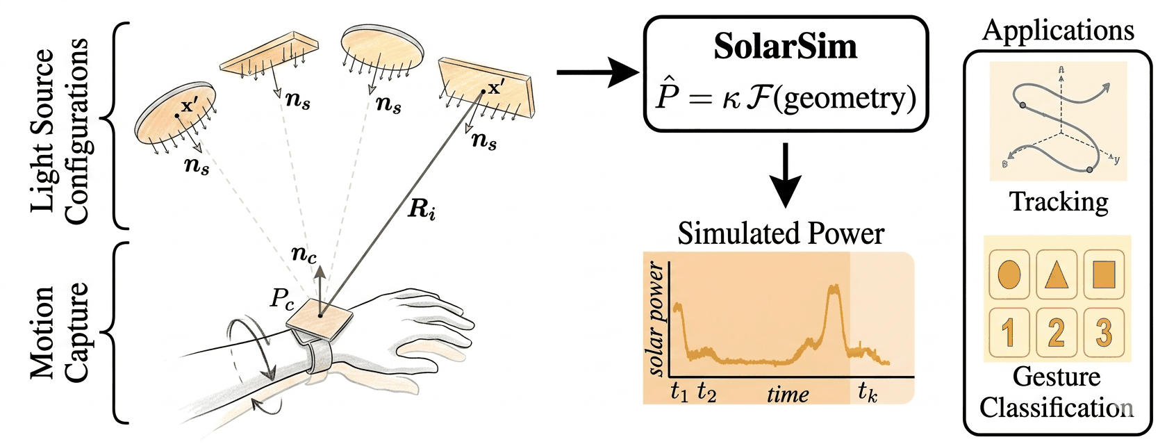
SolarSim pipeline: light source configurations and a wrist motion-capture trajectory feed a radiometric model that outputs a simulated power trace, used for tracking and gesture classification. — **Figure 1.** Given a 3D hand trajectory from motion capture and a light source configuration — emitter geometry, position, and orientation — SolarSim applies a radiometric model to generate a synthetic solar power trace, usable for continuous tracking and gesture classification.

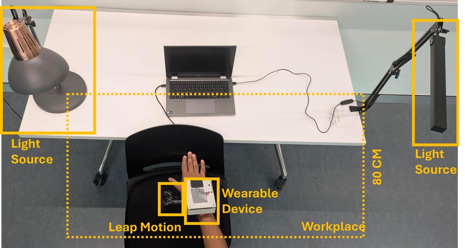
Overhead photograph of the data-collection desk: two light sources, a laptop, a Leap Motion controller, and the wrist-worn solar harvesting device. — **Figure 2.** Data collection setup. A wrist-mounted solar module and IMU are recorded alongside hand position and palm orientation from a Leap Motion controller, under configurable overhead lighting.

The Method

Two inputs, one shared kernel, one calibration scalar

SolarSim takes a motion trajectory and a description of the lighting, and evaluates a radiometric integral for every source in the scene.

1

Motion in

Any motion-capture system supplies timestamped 3D cell positions and outward normals. That is the entire motion input — no IMU, no paired PV recording.

2

View factors

For each source, a radiometric kernel is integrated over the emitter surface, capturing the geometric coupling between source and cell. Purely geometric — no hardware in it.

3

Power out

Per-source view factors are scaled by a calibration constant fit once per environment and summed, yielding the predicted power trace.

Harvested power — superposition over all emitters

P (t) = i = 1 \sum M κ_{i} F_{i} (cell state p_{c} (t), n_{c} (t); source i state p_{s_{i}}, n_{s_{i}}, Γ_{i})

κ_{i}

is a scalar absorbing all hardware and source properties — cell efficiency and area, source intensity, spectral response.

F_{i}

is a purely geometric view factor.

View factor — the shared radiometric kernel

F_{i} = \iint_{A_{i}} K (R_{i}, n_{s_{i}}, n_{c}) \frac{( R _{i} \cdot n _{s_{i}} ) ( - R _{i} \cdot n _{c} )}{∥ R _{i} ∥ ^{4}} d A_{i}, R_{i} = p_{c} - x^{'}

K

encodes inverse-square attenuation and the two cosine projections. It depends only on

R

and the two surface normals — not on the source’s shape.

Circular emitter — polar domain

F_{circ} = \int_{0}^{D /2} \int_{0}^{2 π} K (R_{i} (r^{'}, ϕ)) r^{'} d ϕ d r^{'}

Rectangular emitter — Cartesian domain

F_{rect} = \int_{- L /2}^{L /2} \int_{- W /2}^{W /2} K (R_{i} (u, v)) d u d v

Changing geometry changes only the integration domain $A_{i}$ and its parametrisation of $x^{'}$ . Both integrals are evaluated with Simpson’s rule on a 2D grid.

One kernel, any geometry

The radiometric kernel depends only on the source-to-cell vector and the two surface normals — not on the emitter’s shape. Changing geometry changes only the integration domain and how the surface is parametrised; the kernel is reused unchanged.

Circular sources integrate in polar coordinates, rectangular ones in local tangent coordinates. Both are evaluated with Simpson’s rule on a 2D grid.

Circular — desk lamps, downlights Rectangular — LED panels, troffers Spherical

Calibrating κ

The scalars are estimated once per environment from a short paired motion–PV recording of about 60 seconds, then reused for everything else recorded there.

κ^= ar g κ ⪰ 0 min F κ - P_{2}^{2}

Non-negativity keeps every source’s contribution physical and stops noise being absorbed into offsetting weights. A single emitter reduces to scalar least squares.

Geometry measured once at room setup Re-fit only if lighting is reconfigured

Interactive Demo

Run the physics in your browser

The simulator runs the same radiometric model as the paper. Move the light, pick a gesture, and watch the power trace respond in real time.

Live physics

See geometry become signal

Every peak in the trace is the cell swinging toward the lamp; every trough is it turning away or moving further off-axis. The simulator makes that coupling visible.

Drag the emitter and watch the waveform reshape
Switch between recorded gestures, or draw your own trajectory
Compare simulated output against real recordings
Upload your own motion CSV

Try it out Python package

Findings

What the physics buys you

Validated along two axes: signal fidelity against real measurements across ten emitter configurations, and downstream utility on gesture classification and continuous tracking.

01

Fidelity holds across illumination

Across four source intensities spanning two orders of magnitude and three colour temperatures, correlation stays in a narrow band. Per-environment κ-fitting absorbs both the intensity scaling and the spectral shift, leaving shape fidelity intact.

0.848–0.908ρ, single circular

0.4–40 klxintensity range

2400–6000 Kcolour temperature

02

The kernel is geometry-agnostic

Replacing the circular emitter with a rectangular one swaps the integration domain from polar to Cartesian while reusing the kernel unchanged. Fidelity sits just below the circular range — the kernel transfers across geometry under the same calibration protocol.

0.818ρ, rectangular emitter

0.103nRMSE

03

Multi-emitter scenes compose additively

Two circular emitters at 50 cm and 110 cm separation both land within the single-emitter spread, and pairing a circular with a rectangular source works under the same superposition framework — heterogeneous geometries in one scene, one calibration.

0.810 / 0.817ρ, dual circular

0.800ρ, circular + rectangular

04

Simulation replaces most real training data

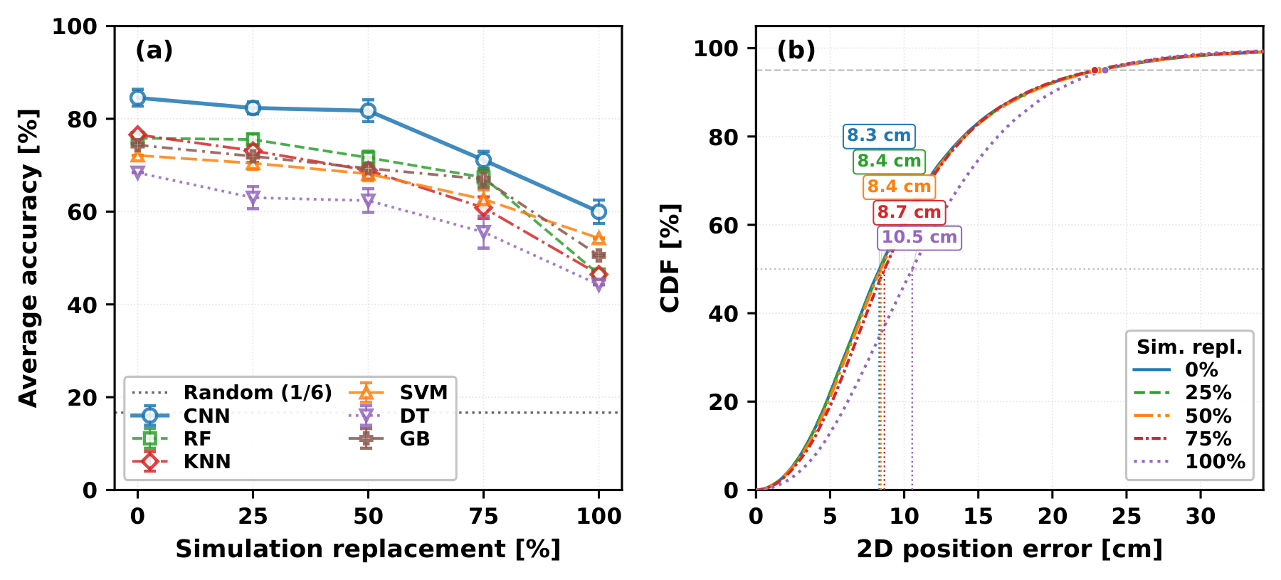
Substituting simulated recordings for real ones degrades tracking remarkably slowly: three quarters of the training set can be synthetic for a 4.1% increase in median error. Classification tolerates half before accuracy moves meaningfully.

+4.1%tracking error at 75% synthetic

8.04 → 8.37 cmmedian 2D error

−3.3%classification at 50% synthetic

05

Physics beats learned simulation at the limit

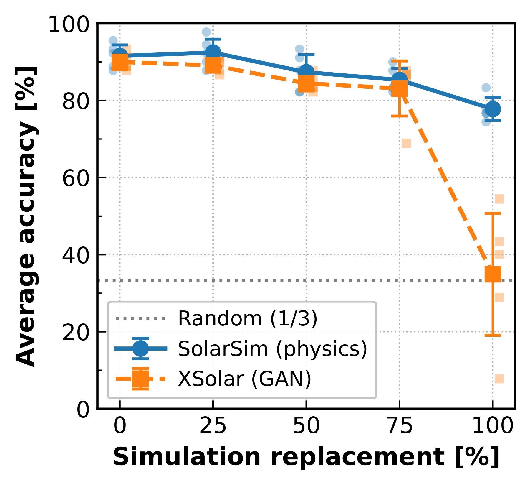
Against XSolar, a conditional GAN that maps IMU to PV, the two stay comparable through 75% substitution. At full replacement they diverge sharply: with no real data to anchor it, the learned distribution collapses toward chance while the physics-based traces preserve class-discriminative structure by construction.

77.8%SolarSim, 100% synthetic

34.9%XSolar (chance = 33.3%)

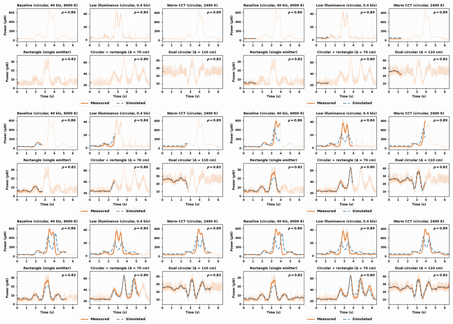
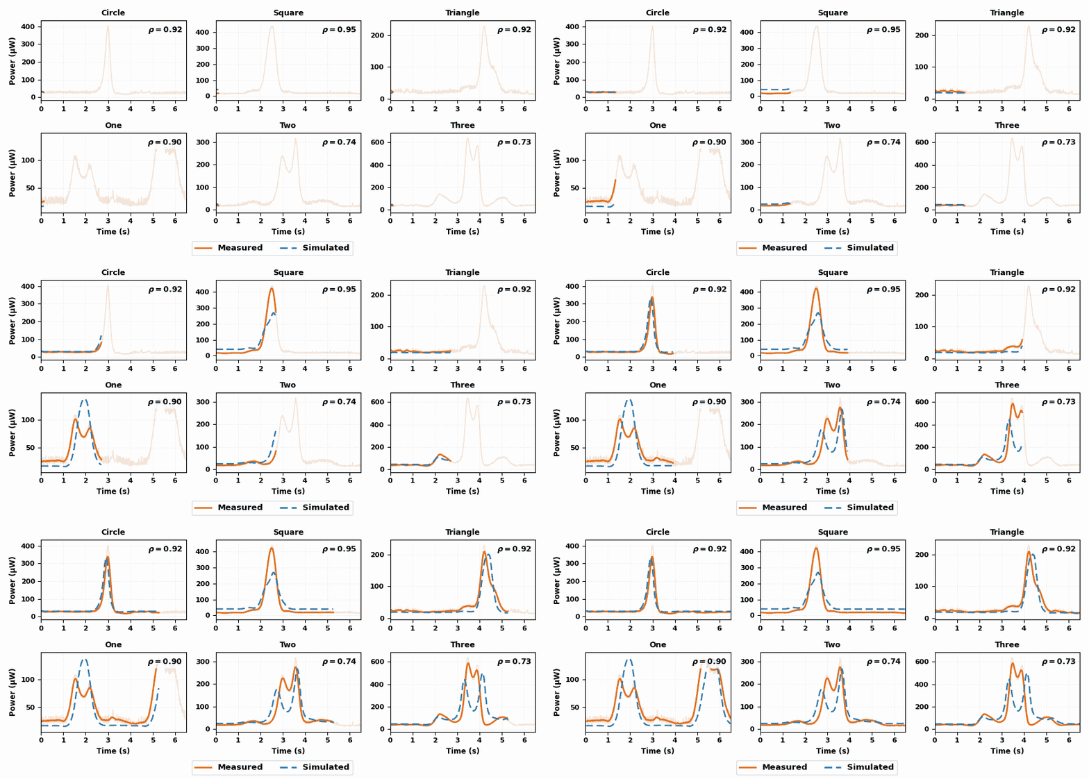
Animation: measured and simulated photovoltaic power drawn over time for six gestures under the baseline configuration. — **Figure 3.** One repetition of each gesture under the baseline configuration, measured against simulated. The faint trace is the raw measurement; the solid line is its denoised form. SolarSim never sees a PV recording — only the trajectory.

Animation: measured and simulated photovoltaic power for gesture Three across six emitter configurations. — **Figure 4.** The same gesture (*Three*) across six emitter configurations, spanning two orders of magnitude in illuminance, three colour temperatures, both emitter geometries, and multi-emitter scenes. Only the scene description changes between panels.

Two panels: classification accuracy versus simulation replacement fraction for six classifiers, and cumulative distribution of 2D tracking error at each replacement level. — **Figure 5.** Effect of synthetic substitution on (a) gesture classification accuracy and (b) hand-tracking position error.

Classification accuracy under substitution comparing SolarSim against the XSolar GAN on a three-class problem. — **Figure 6.** SolarSim against XSolar, a conditional GAN. The two stay comparable through 75% substitution; at full replacement XSolar collapses toward chance while the physics-based traces hold.

Fidelity across every configuration

Configuration	Emitter	CCT / Illuminance	ρ	RMSE (µW)	nRMSE
Baseline	Circular	6000 K / 40 klx	0.861	39.95	0.110
Intensity sweep	Circular	6000 K / 30 klx	0.848	20.04	0.109
Intensity sweep	Circular	6000 K / 15 klx	0.858	17.65	0.116
Intensity sweep	Circular	6000 K / 0.4 klx	0.908	3.20	0.089
Colour temperature	Circular	4000 K / 40 klx	0.867	43.35	0.105
Colour temperature	Circular	2400 K / 40 klx	0.891	43.46	0.097
Geometry	Rectangular	6000 K / 40 klx	0.818	3.36	0.103
Multi-emitter	Dual circular	d = 50 cm	0.810	27.63	0.102
Multi-emitter	Dual circular	d = 110 cm	0.817	5.08	0.100
Multi-emitter	Circular + rect.	d = 70 cm	0.800	8.76	0.113

Where it breaks down

SolarSim assumes line-of-sight propagation, negligible ambient illumination, and no significant interreflections. These hold approximately for wrist-mounted indoor task lighting, but weaken in cluttered or highly reflective environments, and under strong daylight.

The second limitation comes from the motion stream itself. The model depends directly on the estimated cell normal, so under rapid wrist rotation or self-occlusion, pose-estimation quality — not the radiometric formulation — becomes the dominant source of error. This is visible in free-movement recordings, the lowest-fidelity regime we report.

Paper & Resources

Read it, run it, extend it

The simulator, the scene configurations for every illumination setup in the paper, and the recordings are all released.

BibTeX

@inproceedings{ghalwash2026solarsim,
  title     = {SolarSim: Physics-Based Simulation of Wearable Solar
               Harvester Signals for Motion Sensing},
  author    = {Ghalwash, Yasien and Khamis, Abdelwahed and Khalifa, Sara
               and Sandhu, Moid and Jurdak, Raja},
  booktitle = {Proceedings of the ACM on Interactive, Mobile, Wearable
               and Ubiquitous Technologies},
  year      = {2026},
}

Turning motion into solar signals, without collecting any